In-cell drop-down lists are great options to speed up data entry tasks. The data entry operator can enter the required data by simply clicking on a drop-down list and then choosing the correct list item. Most data entry processes utilize drop-down lists to minimize human error and ambiguity in data entry. Continue reading to learn the basics of drop-down lists, the Excel Data Validation tool, and a step-by-step process of adding a drop-down list to your Excel workbook.
What Is an Excel Drop-Down List?
A drop-down list in spreadsheet applications like Excel is a powerful tool to reduce errors and increase productivity. Such functions of the Data Validation tool of Excel reduce error by offering the Excel workbook user some limited list items for a specific cell. When you use Excel for data collection and process the data with a database tool, the drop-down list also helps you to collect uniform data. For example, if the cell only accepts names of fruits, the data entry operator will not be able to add names of animals, fish, spices, etc. The reason is the drop-down menu will only show the listed fruits that your company sells.
The Benefits of a Drop-Down List
Again, the function also increases productivity by automatically suggesting cell items. For example, if the drop-down list has names of 100 employees and the user types “A”, Excel drop-down list will automatically show the names that begin with “A.” Thus, the user can simply select the name using the mouse and save time. If you have noticed here, you can also save yourself from spelling mistakes. Drop-down lists further increase your worksheet’s functionality by offering dynamic report creation. For example, your company operates in 150 countries, there are 200 offices, offices have ten managers each, and each manager controls 20 sales executives. When you need to make a sales report, you can make dependent Excel drop-down lists. A drop-down list for countries will take you to the correct country. Then, choosing an office will show you ten managers who work for that office. And finally, when you pick a manager, you will only see the sales rep who works under that manager. Hence, you do not need to remember the names of all. Just choose a country and follow the multi-tiered drop-down lists.
What Is Data Validation in Excel?
Excel’s cells can take any input, such as characters, numbers, special symbols, etc. However, most processes create a custom-designed worksheet with limited data for each cell in data entry. For example, one cell allows numbers, the next accepts characters, another allows employee names, and so on. But how does Excel enforce all these restrictions? The answer is the Excel Data Validation tool. Most Excel users know this tool as the go-to place to create some quick drop-down menus. However, it has far greater use than the Excel drop-down lists. In a nutshell, whenever the Excel worksheet or workbook administrator wants to force users to enter data in a specific format, they take help from the Data Validation Tool.
Get Familiar With the Data Validation Tool
You can find the Data Validation tool on the Excel ribbon menu. While on an open Excel worksheet, click the Data tab on the ribbon menu. In the Data Tools section, you should find the Data Validation tool. Check the image below to get a clear idea about the tool’s location. When you click the Data Validation button, you will see the Data Validation dialog box with three tabs: Settings, Input Message, and Error Alert.
Settings
Settings lets you customize the options such as allowed data formats and set rules for data entry. The latest Microsoft Excel for desktop or laptop lets you add the following formats:
Any value for no validation.The whole number allows users to enter only whole numbers in the target cell.Decimal lets you format the cell to accept only decimal numbers.The list enables you to create drop-down lists with predefined list items.Date empowers you to restrict specific cells only for entering date values.Time validation formats the target cell to only accept time values.Text length is the perfect function to limit cell data to a specific number of characters or digits.Custom formatting empowers the user to use formulas within validated cells.
The above formatting or validation functions work by using the following validation criteria. And the good thing is that you can customize these validation criteria in a few cases:
“Between” allows numbers that are within a minimum and maximum range.“Not between” is useful when you need to specify that the entered data should not be within a minimum or maximum value.“Equal to” is useful when fixing the input to a specific value.“Not equal to” means the entered data should not be equal to the specified cell value. “Greater than” is used when the input should be greater than a specific value.“Less than” dictates that the entered value should be less than the indicated figure.“Greater than or equal to” means the input value should be equal to or greater than a set value. “Less than or equal to” means the entered value is either lesser or equal to the set value.
Input Message
Data Validation rules are only helpful when you communicate them with the data entry operators. To do this properly, you can use the Input Message feature of Data Validation in Excel. When you use this feature, you can enter a title and a descriptive message about the Data Validation rules. When users hover the cursor over the formatted cell, a context menu will appear with the Input Message. It is worthy to note that this message will not be visible until you take the mouse pointer over the target cell.
Error Alert
When the user makes errors while entering data in a validated cell, you can show Error Alerts to inform the user. You can use any of the following alerts:
StopWarningInformation
Again, you can type a custom title and error message for the above warnings. This way, the user will be informed and will not repeat the mistakes.
Usage of Data Validation in Excel
Create useful drop-down lists to reduce errors and complete data entry faster.Prevent entry of wrong dates due to typo or human error.Only allow uppercase entries for specific situations like UK postcodes, abbreviations, etc.You can reduce the occurrence of duplicate values to zero.Create dependent drop-down lists to filter data in line with a master list.You can use the Data Validation tool functions when you need only text entries for specific cells.You can force the user to only enter numbers and not any texts or symbols for numerical values.Create the project or office schedules only for weekdays.Validate the user’s entry based on another entry made in a different cell of the same worksheet.Force restriction on a digit or character length of any cell.Make data entries containing pre-determined or specific sets of texts for search purposes.Communicate what may have gone wrong to the data entry operator by creating custom error messages.
Create a Drop-Down List Using Excel Data Validation
A drop-down list gives a context menu of usable values or text for a validated cell. Before creating such a list, collect the values or texts in one place. It could be the same workbook, worksheet, or even a completely different Excel file. Here is what you need to do:
Open the Excel app on your PC and type in a list of items you want in the drop-down list. That is also possible if you want to bring items from another sheet, workbook, or file. You simply need to keep those resources accessible.
Once you have found the source of listed items, you can proceed to the actual part of drop-down list creation.
Select a cell where you need to create an Excel drop-down list.Click on the Data tab on the Excel ribbon menu.You should now find the Data Tools section in the middle of the ribbon menu. It offers several data tools like Text to Columns, Flash Fill, Manage Data Model, and Data Validation.You can directly click on the Data Validation icon to open the Data Validation dialog box.
Alternatively, you can click the text Data Validation to open a drop-down menu and select Data Validation again to open the dialog box.
So far, you have successfully opened the Data Validation dialog box. It offers all the functionalities you need to create a simple drop-down list. Here is how:
By default, you will be on the Settings tab of the Data Validation window.Click on the drop-down menu below the text Allow.A context menu should open containing multiple validation formats. Select the List format from this context menu.
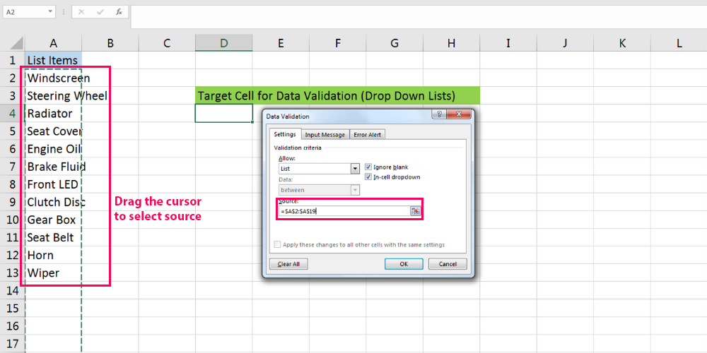
You can not make any changes under the text Data.Below the text Source, you need to enter the source of the list items to display on the drop-down list.Type in the address when selecting a source on another sheet, workbook, or Excel file.Alternatively, to select data sources from the same worksheet, simply click once on the blank field of the source. Then identify the range of cells using the cursor.
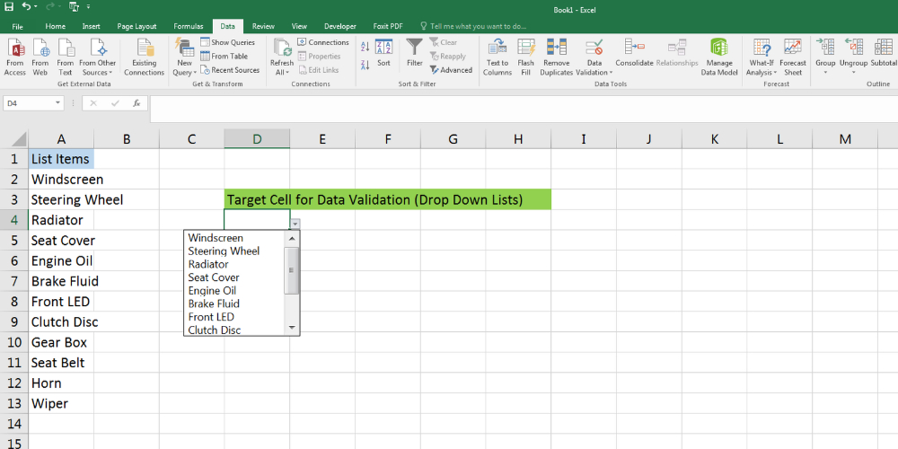
Checkmark Ignore blank and In-cell dropdown options. You may not see the drop-down arrow icon on the validated cells if you uncheck the In-cell dropdown option. Click OK, and your drop-down list is ready.
Creating a Dynamic Excel Drop-Down List
In such a drop-down list, when you select input in one drop-down list, the available data for the second drop-down list automatically changes. Here are the steps to try:
Gather the list of items as shown in the image below. You can also import list items from another workbook or file.
Convert the city names to Named Ranges. To do so, select the cities under a country.
Click on the Name Box and type in the exact country name as it shows in the headers.If trying to use your data, you can follow the same step to convert a list of items under a header into Named Ranges.Create the primary drop-down list using the country name from cell range D1 to G1.
For the Select City column, start creating a drop-down list as usual. In the source, enter the following formula. The idea is to use the INDIRECT formula with a mixed reference for the country drop-down list, which is $A2.
Click Ok to complete the step. Your two-tiered drop-down list is ready.
On this drop-down list, if you select the USA as the country, you will only get USA cities under the Select City column header.
The Final Words
Excel is an excellent tool for data entry and management of numerical data. However, typos can badly hamper your data entry work on Excel. Hence, you need to employ any of the above methods to eliminate human error or typos from data entry. You can follow the simple Excel or dependent drop-down list method. Just look at your data entry process or data collection plan to know which approach to use. You can use this feature almost in any cell. You may also be interested in some free Excel templates for personal budget.


![]()


